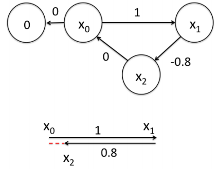
优化问题描述 假设一个机器人初始起点在0处,然后机器人向前移动,通过编码器测得它向前移动了1m,到达第二个地点x1。接着,又向后返回,编码器测得它向后移动了0.8米。但是,通过闭环检测,发现它回到了原始起点。可以看出,编码器误差导致计算的位姿和观测到有差异,那机器人这几个状态中的位姿到底是怎么样的才最好的满足这些条件呢?
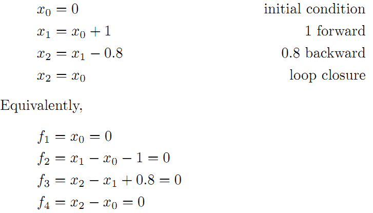
首先构建位姿之间的关系,即图的边:
线性方程组中变量小于方程的个数,要计算出最优的结果,使出杀手锏最小二乘法
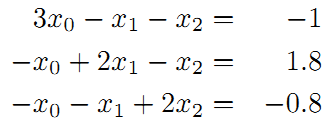
为了使残差平方和最小,我们对上面的函数每个变量求偏导,并使得偏导数等于0.
整理得到:
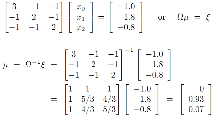
接着矩阵求解线性方程组:
所以调整以后为满足这些边的条件,机器人的位姿为:
可以看到,因为有了x2->x0的闭环检测,几个位置点间才能形成互相约束。这对使用最小二乘解决该优化问题起到了决定性的作用。
该问题描述来源于:https://heyijia.blog.csdn.net/article/details/47686523
下面利用G2O来解上面的问题,以便理解如何使用G2O。
定义顶点 在该问题中,一个位置点就是图优化中的一个顶点。一个顶点可以包含多个需优化量。比如二维环境下的机器人位置一般是3维的(x,y,theta),即一个顶点有三个需要优化的量。
在此问题中,我们只需优化求解一个一维的距离值。即是,一个顶点只包含一个需优化量。
1 2 3 4 5 6 7 8 9 10 11 12 13 14 15 16 17 18 19 20 21 22 23 24 25 26 27 28 29 30 31 32 class SimpleVertex : public g2o::BaseVertex<1 , double > {public : EIGEN_MAKE_ALIGNED_OPERATOR_NEW SimpleVertex (bool fixed = false ) { setToOriginImpl (); setFixed (fixed); } SimpleVertex (double e, bool fixed = false ) { _estimate = e; setFixed (fixed); } virtual void setToOriginImpl () override _estimate = 0 ; } virtual void oplusImpl (const double *update) override _estimate += *update; } virtual bool read (istream &in) return true ;} virtual bool write (ostream &out) const return true ;} };
上面代码中g2o::BaseVertex<1, double>就表示了优化的量是一维的,数据类型是double。
如果查看TEB中设置的优化量,可以发现它是这样写的:
1 g2o::BaseVertex<3 , PoseSE2 >
TEB中的优化量是三维的,即机器人的位姿(x,y,theta)。此处的PoseSE2便是描述机器人位姿的结构体。
自定义一个顶点通常需要重新实现setToOriginImpl()和oplusImpl(const double *update)这两个函数。至于read(istream &in)和write(ostream &out)是为了保存和读取当前顶点数据的。用不上可留空。
setToOriginImpl()函数用于重置顶点的数据。顶点包含的数据变量是_estimate。该变量的类型即是g2o::BaseVertex<1, double>中设置的double。该函数正是用于重置_estimate和使顶点恢复默认状态。
oplusImpl(const double *update)函数用于叠加优化量的步长。注意有时候这样的叠加操作并不是线性的。比如2D-SLAM中位置步进叠加操作则不是线性的。
在此问题中我们是直接线性叠加一维的距离值。
TEB中的位置叠加也是线性叠加的。放置在下面以作参考。
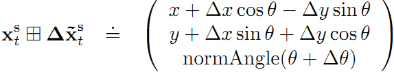
1
2
3
4
5
6
7
8
9
10
11
void plus (const double * pose_as_array) _position.coeffRef (0 ) += pose_as_array[0 ]; _position.coeffRef (1 ) += pose_as_array[1 ]; _theta = g2o::normalize_theta ( _theta + pose_as_array[2 ] ); } virtual void oplusImpl (const double * update) override _estimate.plus (update); }
另外,顶点是可以设置成固定的。当不需要变动某个顶点时,使用setFixed函数来固定。通常,一个优化问题中,至少需要固定一个顶点,否则所有的顶点都在浮动,优化效果也不会好。
定义边 边即是顶点之间的约束。在该问题中就是两位置间的测量值和观测值之间的差值要趋近于0。这里需要定义的边其实就是下面的等式。
实际上,G2O中边有三种:一元边(g2o::BaseUnaryEdge),二元边(g2o::BaseBinaryEdge)和多元边(g2o::BaseMultiEdge)。
1
2
3
g2o::BaseUnaryEdge<D, E, VertexXi> g2o::BaseBinaryEdge<D, E, VertexXi, VertexXj> g2o::BaseMultiEdge<D, E>
不同类型的边有不同数量的模板参数。其中D 是 int 型,表示误差值的维度 (dimension), E 表示测量值的数据类型(即_measurement的类型), VertexXi,VertexXj 分别表示不同顶点的类型。当D为2时,_error的类型变为Eigen::Vector2d,当D为3时,_error的类型变为Eigen::Vector3d。
在上面的约束中,有一个一元边(f1)和三个二元边(f2,f3,f4)。在G2O中可如下定义:
1 2 3 4 5 6 7 8 9 10 11 12 13 14 15 16 17 18 19 20 21 22 23 24 25 26 27 28 29 30 31 32 33 34 35 36 37 38 39 40 41 42 43 44 45 46 47 48 49 50 51 52 53 54 class SimpleUnaryEdge : public g2o::BaseUnaryEdge<1 , double , SimpleVertex> {public : EIGEN_MAKE_ALIGNED_OPERATOR_NEW SimpleUnaryEdge () : BaseUnaryEdge() { } virtual void computeError () override const SimpleVertex *v = static_cast <const SimpleVertex *> (_vertices[0 ]); const double abc = v->estimate (); _error(0 , 0 ) = _measurement - abc; } virtual void linearizeOplus () override _jacobianOplusXi[0 ] = -1 ; } virtual bool read (istream &in) virtual bool write (ostream &out) const }; class SimpleBinaryEdge : public g2o::BaseBinaryEdge<1 , double , SimpleVertex, SimpleVertex> {public : EIGEN_MAKE_ALIGNED_OPERATOR_NEW SimpleBinaryEdge () {} virtual void computeError () override const SimpleVertex *v1 = static_cast <const SimpleVertex *> (_vertices[0 ]); const SimpleVertex *v2 = static_cast <const SimpleVertex *> (_vertices[1 ]); const double abc1 = v1->estimate (); const double abc2 = v2->estimate (); _error[0 ] = _measurement - (abc1 - abc2); } virtual void linearizeOplus () override _jacobianOplusXi(0 ,0 ) = -1 ; _jacobianOplusXj(0 ,0 ) = 1 ; } virtual bool read (istream &in) virtual bool write (ostream &out) const };
因为我们这里测量值是一维的距离值(double类型)而顶点类型为SimpleVertex,所以边需设置成g2o::BaseUnaryEdge<1, double, SimpleVertex>和g2o::BaseBinaryEdge<1, double, SimpleVertex, SimpleVertex>类型。
自定义边同样需要特别关注两个函数computeError()和linearizeOplus()。
computeError()是用于计算迭代误差的。顶点间的约束正是由误差计算函数构建的。优化时误差项将逐步趋近于0。_error的维度和类型通常由构建的模型决定。比如该问题中误差为距离误差。
TEB的速度边构建的误差项为线速度与最大线速度的差值和角速度与最大角速度的差值。所以这里的误差项是二维的。
1
2
3
4
5
6
7
8
9
10
11
12
13
14
15
16
17
18
19
20
21
22
23
24
25
26
27
28
void computeError () { TEB_ASSERT_MSG (cfg_, "You must call setTebConfig on EdgeVelocity()" ); const VertexPose* conf1 = static_cast <const VertexPose*>(_vertices[0 ]); const VertexPose* conf2 = static_cast <const VertexPose*>(_vertices[1 ]); const VertexTimeDiff* deltaT = static_cast <const VertexTimeDiff*>(_vertices[2 ]); const Eigen::Vector2d deltaS = conf2->estimate ().position () - conf1->estimate ().position (); double dist = deltaS.norm (); const double angle_diff = g2o::normalize_theta (conf2->theta () - conf1->theta ()); if (cfg_->trajectory.exact_arc_length && angle_diff != 0 ) { double radius = dist/(2 *sin (angle_diff/2 )); dist = fabs ( angle_diff * radius ); } double vel = dist / deltaT->estimate (); vel *= fast_sigmoid ( 100 * (deltaS.x ()*cos (conf1->theta ()) + deltaS.y ()*sin (conf1->theta ())) ); const double omega = angle_diff / deltaT->estimate (); _error[0 ] = penaltyBoundToInterval (vel, -cfg_->robot.max_vel_x_backwards, cfg_->robot.max_vel_x,cfg_->optim.penalty_epsilon); _error[1 ] = penaltyBoundToInterval (omega, cfg_->robot.max_vel_theta,cfg_->optim.penalty_epsilon); TEB_ASSERT_MSG (std::isfinite (_error[0 ]), "EdgeVelocity::computeError() _error[0]=%f _error[1]=%f\n" ,_error[0 ],_error[1 ]); }
linearizeOplus()函数里主要是配置雅克比矩阵。当然,G2O是支持自动求导的,该函数可以不实现。优化时由G2O自动处理。但准确的实现可加快优化计算的速度。下面介绍雅克比矩阵该如何计算。
计算雅克比矩阵 雅克比矩阵存储了误差项的每一维相对于顶点各优化成员的偏导数。
一元边 一元边只有一个顶点所以只定义了_jacobianOplusXi,其对应顶点类型VertexXi。注意,_jacobianOplus变量才完整地描述雅克比矩阵,_jacobianOplusXi只是_jacobianOplus中相关部分的引用,以方便配置雅克比矩阵。
1 2 3 4 5 6 7 8 9 10 11 12 13 template <int D, typename E, typename VertexXi>class BaseUnaryEdge : public BaseFixedSizedEdge<D, E, VertexXi> { public : using VertexXiType = VertexXi; BaseUnaryEdge () : BaseFixedSizedEdge <D, E, VertexXi>(){}; protected : typename BaseFixedSizedEdge<D, E, VertexXi>::template JacobianType< D, VertexXi::Dimension>& _jacobianOplusXi = std::get <0 >(this ->_jacobianOplus); };
本优化问题的一元边按下面代码的方式计算雅克比矩阵。
1 2 3 4 5 6 7 8 9 10 11 12 13 14 15 16 17 18 19 20 21 22 23 24 25 class SimpleUnaryEdge : public g2o::BaseUnaryEdge<1 , double , SimpleVertex> {public : EIGEN_MAKE_ALIGNED_OPERATOR_NEW SimpleUnaryEdge () : BaseUnaryEdge() { } virtual void computeError () override const SimpleVertex *v = static_cast <const SimpleVertex *> (_vertices[0 ]); const double abc = v->estimate (); _error(0 , 0 ) = _measurement - abc; } virtual void linearizeOplus () override _jacobianOplusXi[0 ] = -1 ; } virtual bool read (istream &in) virtual bool write (ostream &out) const };
二元边 二元边有两个顶点,所以定义了_jacobianOplusXi和_jacobianOplusXj。
1 2 3 4 5 6 7 8 9 10 11 12 13 14 15 16 17 18 template <int D, typename E, typename VertexXi, typename VertexXj>class BaseBinaryEdge : public BaseFixedSizedEdge<D, E, VertexXi, VertexXj> { public : using VertexXiType = VertexXi; using VertexXjType = VertexXj; BaseBinaryEdge () : BaseFixedSizedEdge <D, E, VertexXi, VertexXj>(){}; protected : typename BaseFixedSizedEdge<D, E, VertexXi, VertexXj>::template JacobianType< D, VertexXi::Dimension>& _jacobianOplusXi = std::get <0 >(this ->_jacobianOplus); typename BaseFixedSizedEdge<D, E, VertexXi, VertexXj>::template JacobianType< D, VertexXj::Dimension>& _jacobianOplusXj = std::get <1 >(this ->_jacobianOplus); };
本优化问题的二元边按下面代码的方式计算雅克比矩阵。
1 2 3 4 5 6 7 8 9 10 11 12 13 14 15 16 17 18 19 20 21 22 23 24 25 26 27 28 29 class SimpleBinaryEdge : public g2o::BaseBinaryEdge<1 , double , SimpleVertex, SimpleVertex> {public : EIGEN_MAKE_ALIGNED_OPERATOR_NEW SimpleBinaryEdge () {} virtual void computeError () override const SimpleVertex *v1 = static_cast <const SimpleVertex *> (_vertices[0 ]); const SimpleVertex *v2 = static_cast <const SimpleVertex *> (_vertices[1 ]); const double abc1 = v1->estimate (); const double abc2 = v2->estimate (); _error[0 ] = _measurement - (abc1 - abc2); } virtual void linearizeOplus () override _jacobianOplusXi(0 ,0 ) = -1 ; _jacobianOplusXj(0 ,0 ) = 1 ; } virtual bool read (istream &in) virtual bool write (ostream &out) const };
多元边 多元边直接配置_jacobianOplus变量。
下面的示例代码是teb中的速度约束,来源于edge_velocity.h文件。
1
2
3
4
5
6
7
8
9
10
11
12
13
14
15
16
17
18
19
20
21
22
23
24
25
26
27
28
29
30
31
32
33
34
35
36
37
38
39
40
41
42
43
44
45
46
47
48
49
50
51
52
53
54
55
56
57
58
59
60
61
62
63
64
65
66
67
68
69
70
71
72
73
74
75
76
77
78
79
80
81
82
83
84
85
86
87
88
89
90
91
92
93
94
95
96
97
98
99
100
101
102
103
104
105
106
107
108
109
110
111
112
113
114
115
116
117
118
119
120
121
122
123
124
class EdgeVelocity : public BaseTebMultiEdge<2 , double >{ public : EdgeVelocity () { this ->resize (3 ); } void computeError () { TEB_ASSERT_MSG (cfg_, "You must call setTebConfig on EdgeVelocity()" ); const VertexPose* conf1 = static_cast <const VertexPose*>(_vertices[0 ]); const VertexPose* conf2 = static_cast <const VertexPose*>(_vertices[1 ]); const VertexTimeDiff* deltaT = static_cast <const VertexTimeDiff*>(_vertices[2 ]); const Eigen::Vector2d deltaS = conf2->estimate ().position () - conf1->estimate ().position (); double dist = deltaS.norm (); const double angle_diff = g2o::normalize_theta (conf2->theta () - conf1->theta ()); if (cfg_->trajectory.exact_arc_length && angle_diff != 0 ) { double radius = dist/(2 *sin (angle_diff/2 )); dist = fabs ( angle_diff * radius ); } double vel = dist / deltaT->estimate (); vel *= fast_sigmoid ( 100 * (deltaS.x ()*cos (conf1->theta ()) + deltaS.y ()*sin (conf1->theta ())) ); const double omega = angle_diff / deltaT->estimate (); _error[0 ] = penaltyBoundToInterval (vel, -cfg_->robot.max_vel_x_backwards, cfg_->robot.max_vel_x,cfg_->optim.penalty_epsilon); _error[1 ] = penaltyBoundToInterval (omega, cfg_->robot.max_vel_theta,cfg_->optim.penalty_epsilon); TEB_ASSERT_MSG (std::isfinite (_error[0 ]), "EdgeVelocity::computeError() _error[0]=%f _error[1]=%f\n" ,_error[0 ],_error[1 ]); } #ifdef USE_ANALYTIC_JACOBI #if 0 void linearizeOplus () { TEB_ASSERT_MSG (cfg_, "You must call setTebConfig on EdgeVelocity()" ); const VertexPose* conf1 = static_cast <const VertexPose*>(_vertices[0 ]); const VertexPose* conf2 = static_cast <const VertexPose*>(_vertices[1 ]); const VertexTimeDiff* deltaT = static_cast <const VertexTimeDiff*>(_vertices[2 ]); Eigen::Vector2d deltaS = conf2->position () - conf1->position (); double dist = deltaS.norm (); double aux1 = dist*deltaT->estimate (); double aux2 = 1 /deltaT->estimate (); double vel = dist * aux2; double omega = g2o::normalize_theta (conf2->theta () - conf1->theta ()) * aux2; double dev_border_vel = penaltyBoundToIntervalDerivative (vel, -cfg_->robot.max_vel_x_backwards, cfg_->robot.max_vel_x,cfg_->optim.penalty_epsilon); double dev_border_omega = penaltyBoundToIntervalDerivative (omega, cfg_->robot.max_vel_theta,cfg_->optim.penalty_epsilon); _jacobianOplus[0 ].resize (2 ,3 ); _jacobianOplus[1 ].resize (2 ,3 ); _jacobianOplus[2 ].resize (2 ,1 ); if (dev_border_vel!=0 ) { double aux3 = dev_border_vel / aux1; _jacobianOplus[0 ](0 ,0 ) = -deltaS[0 ] * aux3; _jacobianOplus[0 ](0 ,1 ) = -deltaS[1 ] * aux3; _jacobianOplus[1 ](0 ,0 ) = deltaS[0 ] * aux3; _jacobianOplus[1 ](0 ,1 ) = deltaS[1 ] * aux3; _jacobianOplus[2 ](0 ,0 ) = -vel * aux2 * dev_border_vel; } else { _jacobianOplus[0 ](0 ,0 ) = 0 ; _jacobianOplus[0 ](0 ,1 ) = 0 ; _jacobianOplus[1 ](0 ,0 ) = 0 ; _jacobianOplus[1 ](0 ,1 ) = 0 ; _jacobianOplus[2 ](0 ,0 ) = 0 ; } if (dev_border_omega!=0 ) { double aux4 = aux2 * dev_border_omega; _jacobianOplus[2 ](1 ,0 ) = -omega * aux4; _jacobianOplus[0 ](1 ,2 ) = -aux4; _jacobianOplus[1 ](1 ,2 ) = aux4; } else { _jacobianOplus[2 ](1 ,0 ) = 0 ; _jacobianOplus[0 ](1 ,2 ) = 0 ; _jacobianOplus[1 ](1 ,2 ) = 0 ; } _jacobianOplus[0 ](1 ,0 ) = 0 ; _jacobianOplus[0 ](1 ,1 ) = 0 ; _jacobianOplus[1 ](1 ,0 ) = 0 ; _jacobianOplus[1 ](1 ,1 ) = 0 ; _jacobianOplus[0 ](0 ,2 ) = 0 ; _jacobianOplus[1 ](0 ,2 ) = 0 ; } #endif #endif public : EIGEN_MAKE_ALIGNED_OPERATOR_NEW };
上面的代码中_error[0]对应线速度vel误差,_error[1]对应角速度omega误差。所以需要求解vel和omega分别相对于顶点变量x,y,theta的导数。
_jacobianOplus[0].resize(2,3);对应第一个顶点,其中误差项有两维,顶点优化变量有3维,所以雅克比矩阵是一个2x3的矩阵。
_jacobianOplus[1].resize(2,3);对应第二个顶点,其中误差项有两维,顶点优化变量有3维,所以雅克比矩阵是一个2x3的矩阵。
_jacobianOplus[2].resize(2,1);对应第三个顶点,其中误差项有两维,顶点是时间差,只有一维,所以雅克比矩阵是一个2x1的矩阵。
创建优化器 1 2 3 4 5 6 7 8 9 10 typedef g2o::BlockSolver<g2o::BlockSolverTraits<1 , 1 >> BlockSolverType; typedef g2o::LinearSolverDense<BlockSolverType::PoseMatrixType> LinearSolverType; auto solver = new g2o::OptimizationAlgorithmGaussNewton ( g2o::make_unique <BlockSolverType>(g2o::make_unique <LinearSolverType>())); g2o::SparseOptimizer optimizer; optimizer.setAlgorithm (solver); optimizer.setVerbose (true );
teb中的优化器设置
1 2 3 4 5 6 7 8 9 10 11 12 13 14 15 16 17 18 19 20 21 22 23 24 25 26 27 28 29 30 31 typedef g2o::BlockSolverX TEBBlockSolver;typedef g2o::LinearSolverCSparse<TEBBlockSolver::PoseMatrixType> TEBLinearSolver;std::shared_ptr<g2o::SparseOptimizer> TebOptimalPlanner::initOptimizer () static std::once_flag flag; std::call_once (flag, [this ](){this ->registerG2OTypes ();}); std::shared_ptr<g2o::SparseOptimizer> optimizer = std::make_shared <g2o::SparseOptimizer>(); auto linearSolver = std::make_unique <TEBLinearSolver>(); linearSolver->setBlockOrdering (true ); auto blockSolver = std::make_unique <TEBBlockSolver>(std::move (linearSolver)); g2o::OptimizationAlgorithmLevenberg* solver = new g2o::OptimizationAlgorithmLevenberg (std::move (blockSolver)); optimizer->setAlgorithm (solver); optimizer->initMultiThreading (); return optimizer; }
从上面的代码对比可以看出,BlockSolver可设成固定的,也可以设成动态的。
下面是本人对于BlockSolver设置的理解,不一定正确。仅为参考。
优化变量的维度通常是明确的,但误差项的维度可能是变化的。每条边的误差项维度可能都不一样。这时应该使用g2o::BlockSolverX,以便能动态适应误差项的维度。
linear solver也是可选的。主要有下面几种可选:
1
2
3
4
5
g2o::LinearSolverCSparse g2o::LinearSolverCholmod g2o::LinearSolverEigen g2o::LinearSolverDense g2o::LinearSolverPCG
不同的linear solver有不同的依赖,需要注意是否已经安装了相应的依赖。
添加顶点 1 2 3 4 5 6 7 8 9 10 11 12 13 14 15 16 17 18 19 20 21 22 23 std::vector<SimpleVertex *> vertexs; SimpleVertex *v = new SimpleVertex (); v->setEstimate (0 ); v->setId (0 ); v->setFixed (true ); optimizer.addVertex (v); vertexs.push_back (v); SimpleVertex *v1 = new SimpleVertex (); v1->setEstimate (1 ); v1->setId (1 ); optimizer.addVertex (v1); vertexs.push_back (v1); SimpleVertex *v2 = new SimpleVertex (); v2->setEstimate (0.1 ); v2->setId (2 ); optimizer.addVertex (v2); vertexs.push_back (v2);
顶点的id需要确保不能重复。
顶点可使用setEstimate接口设置初始值。
添加边 1 2 3 4 5 6 7 8 9 10 11 12 13 14 15 16 17 18 19 20 21 22 23 24 25 26 27 28 29 30 31 32 SimpleUnaryEdge *edge = new SimpleUnaryEdge (); edge->setVertex (0 , vertexs[0 ]); edge->setMeasurement (0 ); edge->setInformation (Eigen::Matrix<double , 1 , 1 >::Identity ()); optimizer.addEdge (edge); SimpleBinaryEdge * edge1 = new SimpleBinaryEdge (); edge1->setVertex (0 , vertexs[1 ]); edge1->setVertex (1 , vertexs[0 ]); edge1->setMeasurement (1 ); edge1->setInformation (Eigen::Matrix<double , 1 , 1 >::Identity ()*1.0 ); optimizer.addEdge (edge1); SimpleBinaryEdge * edge2 = new SimpleBinaryEdge (); edge2->setVertex (0 , vertexs[2 ]); edge2->setVertex (1 , vertexs[1 ]); edge2->setMeasurement (-0.8 ); edge2->setInformation (Eigen::Matrix<double , 1 , 1 >::Identity ()); optimizer.addEdge (edge2); SimpleBinaryEdge * edge3 = new SimpleBinaryEdge (); edge3->setVertex (0 , vertexs[2 ]); edge3->setVertex (1 , vertexs[0 ]); edge3->setMeasurement (0 ); edge3->setInformation (Eigen::Matrix<double , 1 , 1 >::Identity ()); optimizer.addEdge (edge3);
边也有setId接口,但不设置好像也可以。如果设置也需确保不重复。但id号的顺序似乎并没有要求。
使用setVertex接口设置顶点时是有顺序的。这个顺序与边的computeError函数中使用顶点的顺序要对应起来。
setMeasurement接口用于设置内部的_measurement值。
setInformation接口用于设置信息矩阵。信息矩阵是方正矩阵,其行列数由误差项的维度决定。
1 2 3 4 5 6 7 8 9 10 11 12 13 14 15 16 17 18 19 20 21 22 23 24 25 26 27 void TebOptimalPlanner::AddEdgesVelocity () if (cfg_->robot.max_vel_y == 0 ) { if ( cfg_->optim.weight_max_vel_x==0 && cfg_->optim.weight_max_vel_theta==0 ) return ; int n = teb_.sizePoses (); Eigen::Matrix<double ,2 ,2 > information; information (0 ,0 ) = cfg_->optim.weight_max_vel_x; information (1 ,1 ) = cfg_->optim.weight_max_vel_theta; information (0 ,1 ) = 0.0 ; information (1 ,0 ) = 0.0 ; for (int i=0 ; i < n - 1 ; ++i) { EdgeVelocity* velocity_edge = new EdgeVelocity; velocity_edge->setVertex (0 ,teb_.PoseVertex (i)); velocity_edge->setVertex (1 ,teb_.PoseVertex (i+1 )); velocity_edge->setVertex (2 ,teb_.TimeDiffVertex (i)); velocity_edge->setInformation (information); velocity_edge->setTebConfig (*cfg_); optimizer_->addEdge (velocity_edge); } } ... }
最终优化求解的结果为estimated model: 0 0.933333 0.0666667 。基本和标准结果一致。
如果将edge1的信息矩阵如下设置:
1 edge1->setInformation (Eigen::Matrix<double , 1 , 1 >::Identity ()*10.0 );
优化求解的结果为:estimated model: 0 0.990476 0.0952381
可以发现x1更接近1了。说明此时我们更相信编码器测量的从x0到x1的距离值。
完整的测试代码可查看下面的链接:
https://github.com/shoufei403/g2o_learning.git
觉得有用就点赞吧!
我是首飞,一个帮大家填坑 的机器人开发攻城狮。
另外在公众号《首飞 》内回复“机器人”获取精心推荐的C/C++,Python,Docker,Qt,ROS1/2等机器人行业常用技术资料。